Fireworks

January 7, 2026

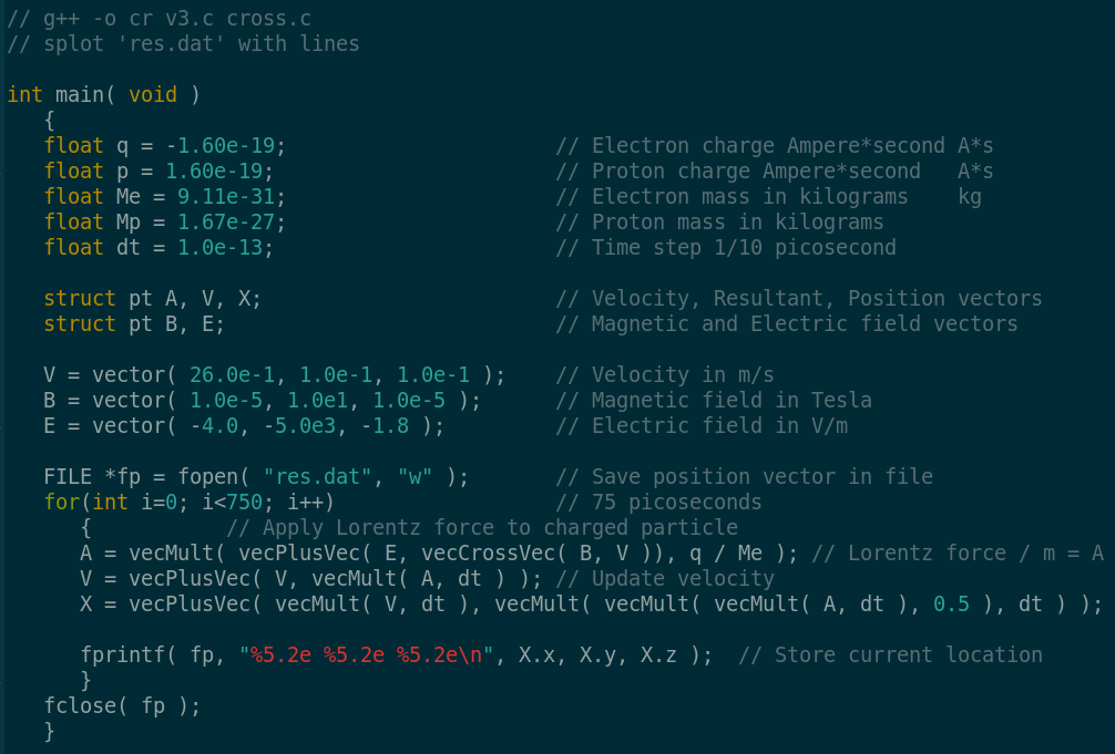
I was curious how an electron moves in a magnetic field. So I dug out my physics books and worked some problems. After reviewing the basics I settled on the Lorentz force equation. Force = q ( E + V cross B ). Here q is the charge of an electron, E is the electric field vector, V is the velocity vector, and B is the magnetic field vector. I use + to represent vector addition, and cross to represent the cross product between V and B. Multiplying a vector by a scalar was implied when the charge was applied to the vector. Now that I had my equation I needed to find out how it responded to various inputs. I wrote a little code to generate test data.

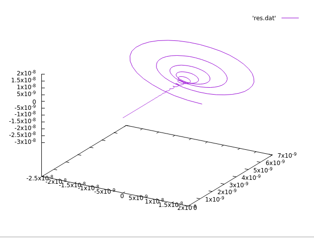
I used gnuplot to give me this image of 75 picoseconds of data. An electron captured by earth's magnetic field cycles from one pole to the other 5 to 10 times each second. I expect there is a persistent hum at that radio frequency. The antenna required to hear it would be rather long :)

This let me find a useful time interval. I chose 1/10 of a picosecond as dt, or 10^-13 seconds. I wrote some more code and got the Lorentz() function working in my 3D graphics environment.

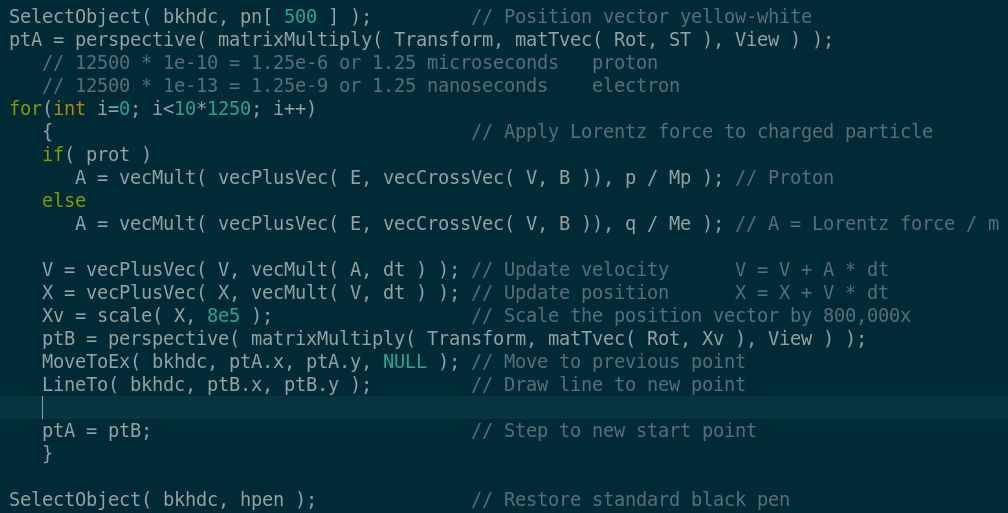
The Lorentz force equation requires three vectors: velocity, magnetic, and electic. The X component of the electic field, E.x, automatically sweeps from -30,000 to 30,000 volts and back again. This gives the simulation the character of a metronome. Both V and B vectors respond to keystrokes from the user.

The magnetic vector, B, begins at 1 Gauss, 1e-5 Tesla, for each component. This is an artifact of having both apps running in concert with one another. Hit the F key to step the B.y component value. The magnetic field now points down, similar to the Earth's magnetic field. Once you have stepped the magnetic vector it never returns to the 1 Gauss setting. It steps by 0.2 Tesla until it reaches 3.6 Tesla. Then it returns to 0.0, with 1e-5 Tesla for the other coordinates.

The V key controls the X component of the velocity vector. Each time you hit it the velocity increases by a factor of ten. V.x begins at 2.6e-2, 0.026 meters/second or 26 millimeters/second. Keep hitting the V key to achieve ever greater velocity. The limit is 2.6 million meters/second, which is sufficient for this exercise; to find the limits of interest of the Lorentz function.

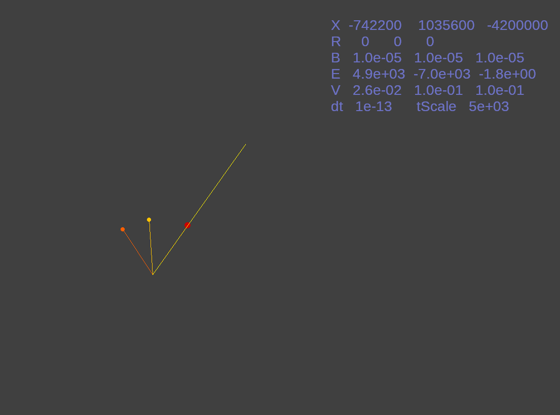
Here is Lorentz() with its initial settings. A magnetic field of 1 Gauss pointing in the X,Y,Z direction diagonally across a cube. The magnetic field vector is designated by an orange line terminated with an orange ball. The yellow line and ball designate the velocity vector. Lastly we have the electric vector which is designate with a red line and ball. The lighter yellow line is the resultant of these three vectors after the Lorentz force is applied.

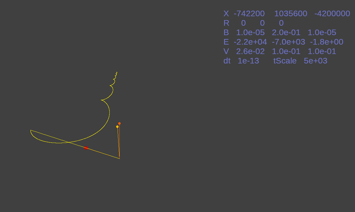
This is after the magnetic force has been increased to 0.2 Tesla. Notice the electron's circuitous path created from the three vector values.

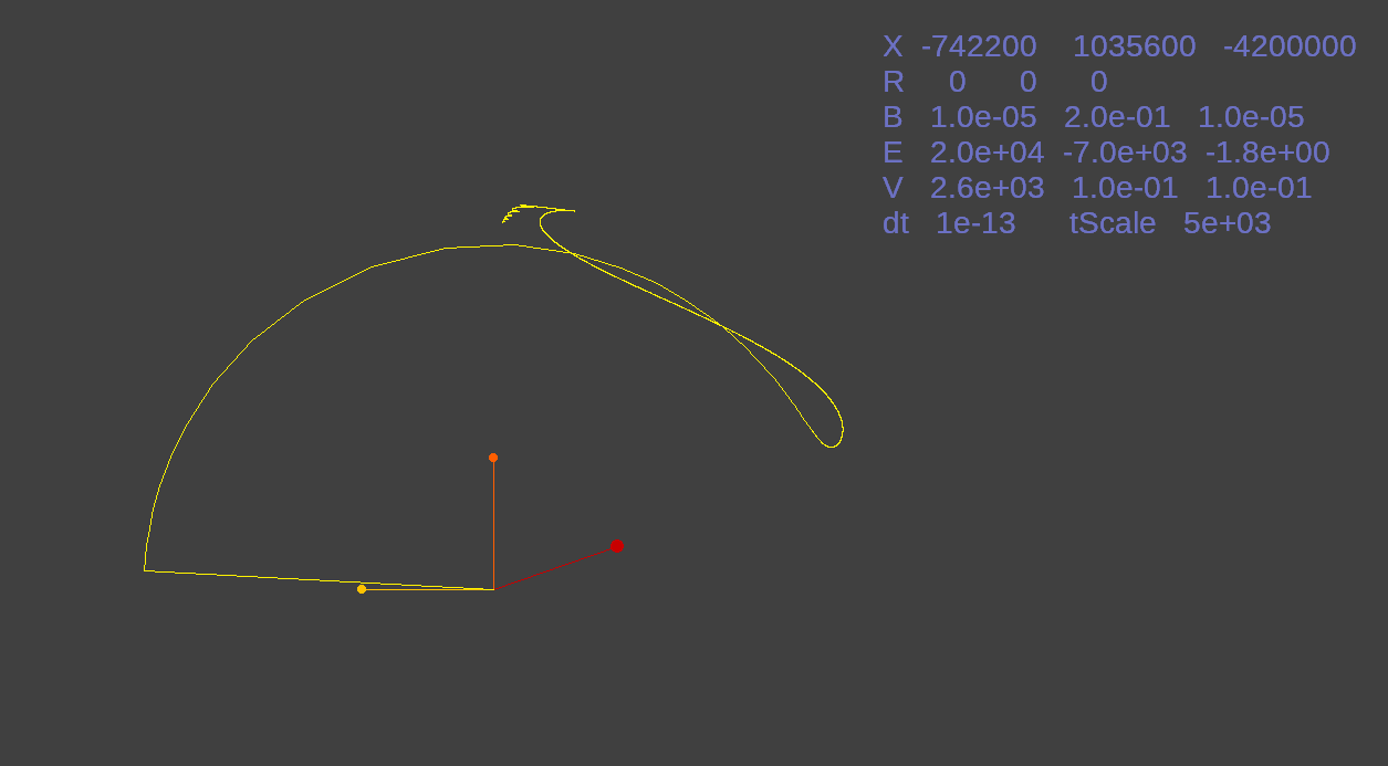
Here I increased the velocity to 2,600 meters per second under 0.2 Tesla of magnetic force.

Next I hit the END key to change to a top view of the vectors with the same settings as the previous image.

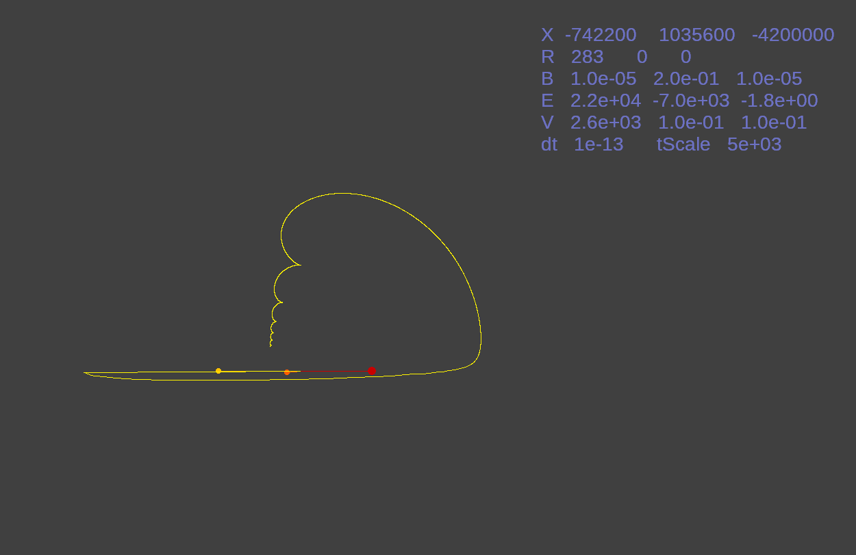
While the field settings remain the same I hit the P key to change to a proton instead of an electron. Notice the time scale changes. Instead of 1/10 of a picosecond interval I now use 1/10 nanosecond for the slower, more massive particle.

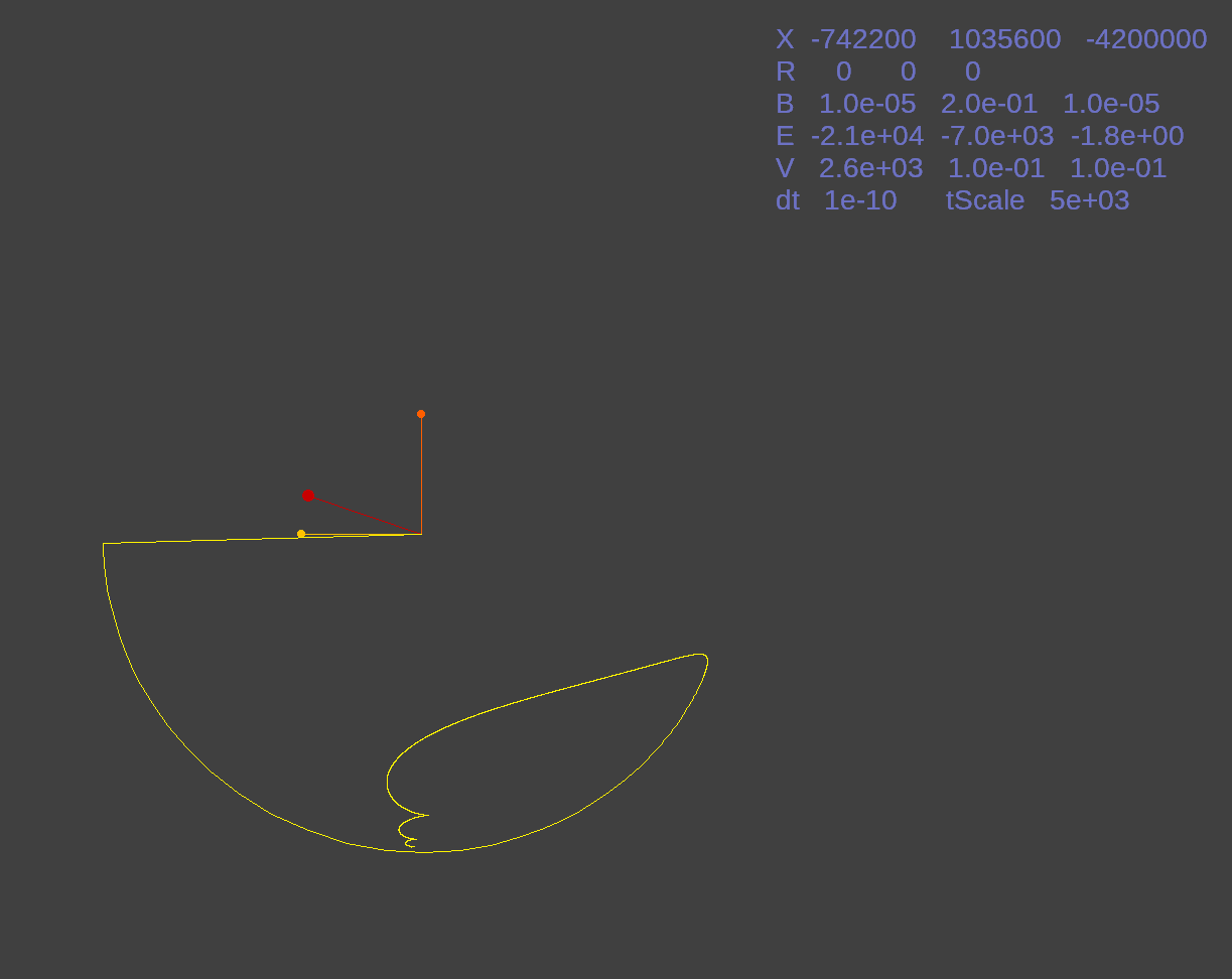
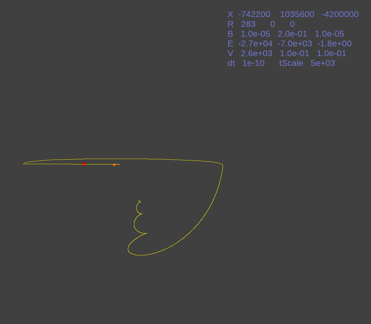
Lastly I hit the HOME key to provide a side view of the proton's motion.

This is a short animation of Lorentz() as it sweeps the electric vector from -30,000 to 30,000 volts and back again. While the V and B vectors are controlled by the user's keystrokes, the E vector is autonomous.

I also hit the Y key so the animation autorotates around the Y axis. I can rotate the view around any of the three major axes by hitting the X, Y, or Z key (or all three for chaotic motion). Rotation helps me see the various effects more easily. This is especially helpful for the orbital simulation featured next.

Toward the end I hit P. Watch for the time change and the orientation of the path with respect to the magnetic field. A proton is much more massive so it takes longer for it to respond to the effects of the fields. I changed perspective by three orders of magnitude. However, both are at Scalosian speeds.

I hope to use the continuous color change in my magnetic field lines. The color index can change as more, or fewer, electrons impinge upon it.

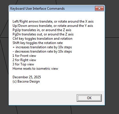
This is the help dialog box of my now standard keyboard user interface.

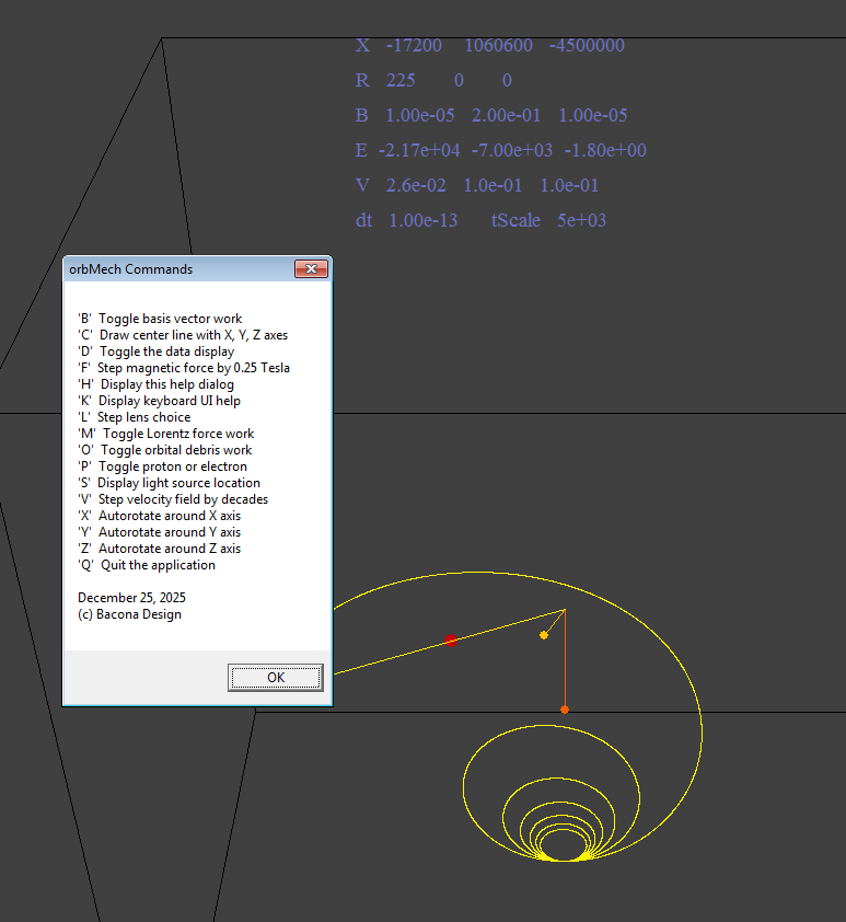
These are the keys which control application specific settings.

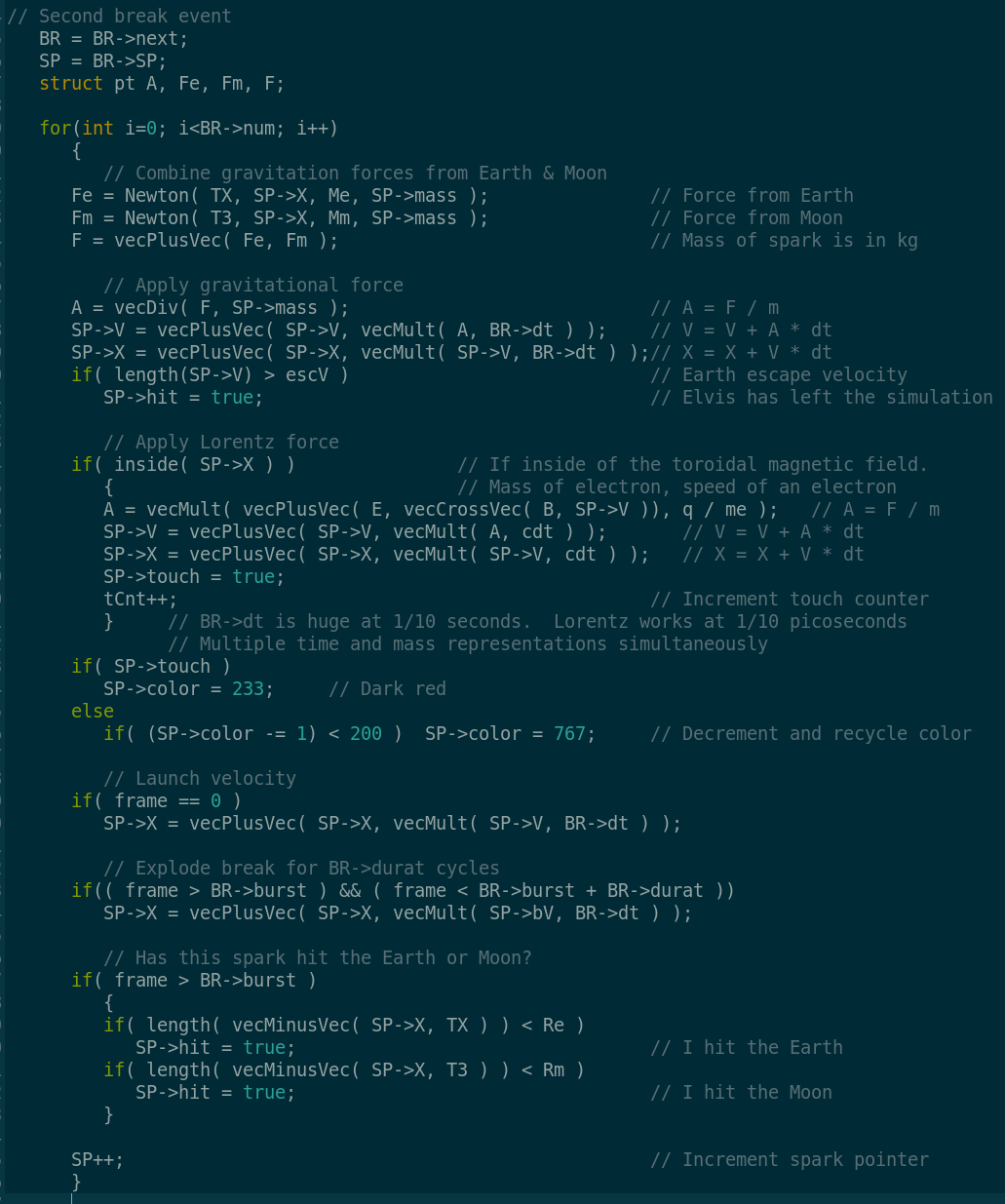
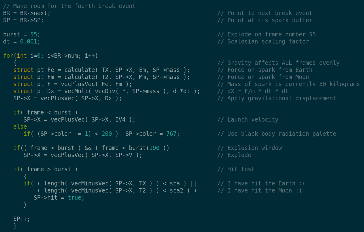
Notice how the break behavior is changing. The force of gravity on each particle is calculated for both the earth and the moon. Then they are summed and Newton's laws of motion are applied to find the new location. Next the Lorentz force is calculated if the particle (electron) is inside of the earth's magnetic field, designated by the torus. Once the force is determined Newton's laws of motion are applied again.

If the electron visits the magnetic field it is marked with a steady color. Since I am only interested in what happens inside the field this lets me keep track of those particles. Launch velocity places the particle at its initial location relative to the earth. Then at a given time it explodes radially outward at its break velocity. I made sure this was large enough to travel across earth's orbit. This gave me the most particles interacting with the magnetic field. If the break is too slow or too fast I get fewer particles hitting the magnetic field. Or they all hit the earth and exit the simulation.

Lastly, we check if the particle has hit either the earth or the moon. If it has hit either of them it is no longer displayed during the simulation.

Lorentz force in space.

January 10, 2026

I decreased the mass of each particle by four orders of magnitude. I also changed color recycling to set the color when it is inside the magnetic field. Then the color fades with time. When it drops to a dull red the color index resets to its individual upper limit. I am testing the index range for best appearance.

January 11, 2026

I found some data files which outline the continents at three resolutions. I first mapped the data using a Mercator projection. Then I put the map back onto a spherical globe and animated it.

December 5, 2025

December 4, 2025

December 2, 2025

November 20, 2025