Ecology Simulation
August 26th, 2025
Download pdf: How to Build an Ecosystem
Download executable: ecoDraw.exe
Download source code: ecoDraw.c
How to Build an Ecosystem
I use genetic algorithms to breed an ecosystem full of plants, herbivores, and carnivores living on energy from a nutrient layer. In nature there are many levels of carnivores with competition among various herbivores. I implemented only one species at each level to simplify my work. I use three genetic operators in the simulation: crossover, mutation, and selection. Survival is my sole selection criterion. If an organism has enough energy it survives. If it has enough more it can reproduce. It finds a mate with whom it exchanges genetic material. Copies of two parent chromosomes are combined using the crossover operator with a small amount of mutation. The upper bits from one parent and the lower bits from the other parent form the new chromosome. This process is repeated for all chromosomes in each parent. Each organism has an energy and a marker chromosome. Every plant also has a chromosome to hold its characteristic traits. Herbivores have a chromosome to store their traits, while carnivores have a chromosome to hold theirs. Crossover breeds for the most fit organisms; mutation breeds for change.
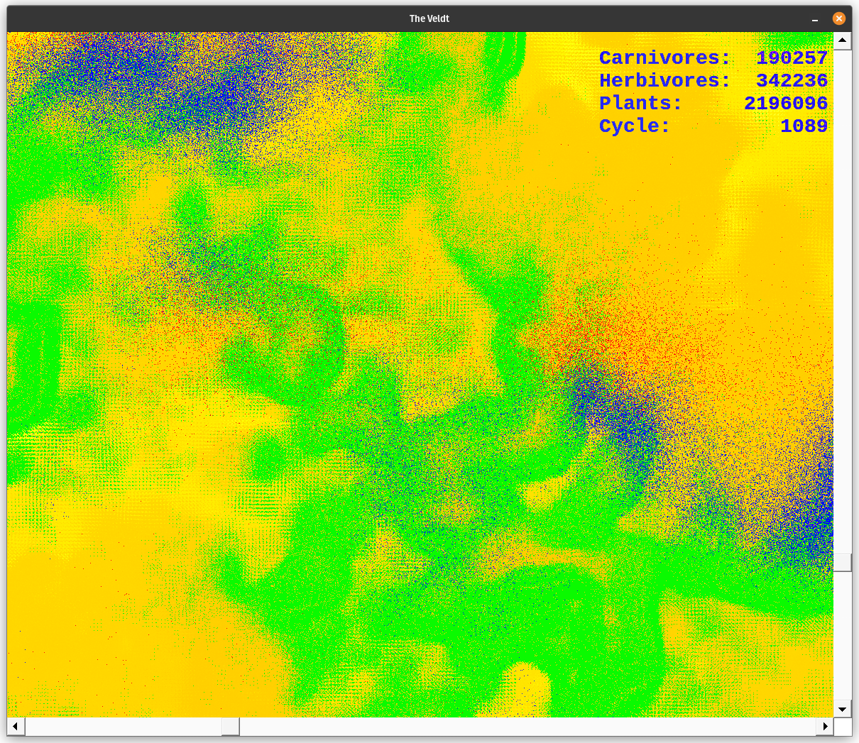
The environment lives in a 3500x3500 pixel area which I call The Veldt. The nutrient layer is a grid which forms the framework of the ecosystem. Each organism: plant, herbivore, or carnivore lives at a point on that grid. The plants feed from the nutrient layer at their location. Herbivores and carnivores have other feeding behaviors. The plants absorb the nutrients then reproduce, if given enough energy. The herbivores move around the veldt searching for plants to eat. The carnivores follow herbivores; if they are hungry they feast. Scroll around the environment using the arrow keys, or the scroll bars. PgUp and PgDn, or the mouse wheel can also control up and down movements.
I wrote this simulator to examine how energy flows through the system. The ecosystem starts with the energy contained in each organism and stored in the nutrient layer. Each organism expends energy during a cycle. The rate of metabolism is determined by a gene on the organism's energy chromosome EN. Herbivores and carnivores do not use all the available energy when they eat. The amount they absorb is determined by another gene on the EN chromosome. Any left over plant or herbivore energy flows back into the nutrient layer. Reproduction is similarly messy. Each parent provides one half of the offspring's natal energy. They also return a certain amount of energy back to the nutrient layer. At senescence an organism dies and its energy flows to the nutrient layer.
During each time cycle every plant eats, reproduces (if energetic enough), and dies if its energy drops below zero. Each herbivore and carnivore moves around, eats what it can, reproduces if possible, and dies if it must. The herbivores and carnivores move directed by their direction chromosome DR. The DR chromosome has eight genes which represent possible directions, plus another for speed. The genes on DR are read and a normalized direction vector is calculated.
Plants have spines and poison, determined by genes on the plant chromosome PL. Herbivores can eat some level of poison and shorter spines, both genes are stored on the herbivore chromosome HB. Reproduction age, satiety, and senescence are also genetically determined. Use the two-click spot sample mechanism to track certain genes and see histograms of some traits. Approximately one half of the genes are currently expressed. All of the energy and direction genes are employed, but only some of the plant, herbivore, and carnivore genes are accessed. Those genes describe behavior traits. At the present I am not using the sensor chromosome SN. All five senses could improve the hunting skills of a carnivore, or provide some level of safety to a herbivore.
Energy flow
The nutrient layer begins with a uniform amount of energy in each cell of the grid. Each plant, herbivore, and carnivore is created with a fixed amount of energy. Each organism gains energy by absorbing energy. All organisms lose energy to the environment because of their metabolism. Herbivores and carnivores also lose energy when they move. If an organism reaches the age of senescence it dies, giving its remaining energy back to the environment.
A plant absorbs energy from the nutrient layer. It examines its satiety gene (EN::G3) to determine whether it is hungry or not. If it is hungry then it looks at its absorb gene (EN::G4) to calculate the absorption factor. Each plant gains absorb * E(i,j)->energy. In other words, it absorbs a certain percentage of the nutrients available at E(i,j).
Herbivores express seven genes when they feed. In order: speed (DR::G0), satiety (EN::G3), eat (HB::G1), resist (HB::G0), spine (PL::G1), strength (PL::G2), and absorb (EN::G4). On a side note: examine the labels inside the parentheses. The first two characters (EN, DR, HB, and PL) designate which chromosome is used. The final two characters: G0, G1, etc. designate which gene on the chromosome is used. It is a shorthand I use to help me map genes.
Each organism has an energy chromosome, EN. It determines the energy use per cycle, the energy absorption rate, the satiety level, the breeding age, and the age of senescence. After many tests I have found it is best to not allow eternal life. It is also not good to overeat. Thus the two genes: senescence and satiety. If a herbivore is hungry it eats until full. If it is already full it does not eat any more.
Animals are messy during feeding. Not all of their food gets eaten, some of it falls onto the ground, and then back to the nutrient layer. The herbivore absorbs a genetically determined percentage of the plant's energy (EN::G4). The rest returns to the nutrient layer while the plant is removed from the simulation. Carnivores absorb energy by eating herbivores. EN::G4 determines how much energy the carnivore gains. The herbivore's remaining energy returns to the environment at its location.
I expressed a few more genes so plants now have both spines and poison. Reciprocally, each herbivore has two genes which allow them to withstand a certain amount of poison, or a certain length of spines. I find it interesting to see how plants breed toward more spines or higher poison levels, while the herbivores breed for higher resistance to poison and the ability to eat longer spines. Use the two-click spot sampling mechanism; then click the 'Spine War' button to monitor the progress.
When an organism reproduces it must have enough energy, and be old enough. Two plants breed to create an offspring with 1/8 of the energy from both parents. Each parent also loses 1/16 of their energy back to the environment. That means each parent loses 3/16 of their energy due to reproduction. So the energy for each offspring is taken from both parents while some energy falls back into the environment. No energy is created and hopefully none is lost. It would be good to monitor the energy total from nutrient layer up through the carnivore layer. Ideally, the total will be a fixed amount.
It is easy to track the history of energy use in the nutrient layer. A large growth of plants is followed by a dark, depleted nutrient layer. Watch the herbivores eat a dense area of plants. Notice the nutrient layer growing brighter as the plants disappear. When the carnivores start feasting on those herbivores the nutrient layer grows even brighter. All of the waste energy from eating, and reproduction, is fed directly to the nutrient layer. This is recorded in the nutrient layer until the next wave of growth passes through.
The nutrient layer, and each organism, starts with a set amount of energy. All of the organisms metabolize, each loses energy and grows one cycle older. The metabolic energy is returned evenly across the nutrient layer. Balancing the energy flow makes the system more stable for longer simulation runs.
Simulation display
The application begins with a window 1000x1000 pixels in size. It is set to the upper right of the 3500x3500 pixel simulation area. Scroll across the area to find points of interest. Expand the window to fit your screen size. A text window also opens. It displays the cycle number; plant, herbivore, and carnivore populations; as well as the highest energy level of the plants, herbivores, and carnivores. I use this display to tune the ecosystem. I also graph the information it stores in dt.dat with Gnuplot so I could see population or energy cycles.
The simulation uses the following colors. Each red pixel represents a single carnivore, each blue pixel is a herbivore, and each green pixel represents a plant. The nutrient layer is displayed a little differently. Each pixel represents the energy level at that location. The darker color (a dusky brown shade) is shown where the energy has been depleted. The lightest colors represent areas of high energy. Notice how rapidly plants reproduce where the color is bright, as compared to areas where the nutrient layer is depleted, designated by darker colors. The nutrient layer maps a 'history' of energy use.
Over time the nutrient layer develops a complex, mosaic structure. This variation is mirrored by the plant, herbivore, and carnivore populations. Noticing this caused me to save mature nutrient layer data for the future. Hit the 'n' key at any time to store a new copy of nut.dat, the entire nutrient layer energy level map.
The application searches for two files when the simulation begins. One of them is the nutrient layer data, nut.dat. The other is the organism sample file, sample9GM.dat. This is a sample taken every 1000 cycles of the surviving organisms. The organisms become better adapted to the system as the simulation matures. Storing both the nutrient layer and the organism samples, lets me save the genetic information and the nutrient mosaic. If both of the files are present the ecosystem begins with a varied mosaic of nutrients, and time tested chromosomes. Because these are only sample files, new, random organisms are added to achieve the initial population levels. Thus mature genetics is represented by the sampled organisms, while random genetics is provided to the remaining population. The simulation begins with a uniform nutrient layer if the nutrient data is not available.
Genes from bits to behavior
Organisms derive traits from genes mapped on chromosomes. All genes are bit based. Trait parameters are calculated from those binary genes. Each organism has multiple chromosomes, each of them holds multiple genes. Every chromosome is 32 bits long. I employ a few simple techniques to convert genes into trait parameters. I will use the direction gene DR as an example. DR has 9 genes mapped onto it. 3 bits for each cardinal direction (N,NE,...,W,NW) and 3 more for a speed gene. I sum the 8 raw direction values, then divide each value by that sum for a direction probability. One herbivore's direction vector gives me: E 0.125, SW 0.250, S 0.125, SE 0.500. This herbivore is able to move in four directions: E, SW, S, and SE. It moves southeast one half of the time, southwest one quarter of the time, and it moves east or south one eighth of the time respectively. This herbivore cannot move in any of the other four directions.
I have written a number of ecology simulations. In those earlier simulations I expressed genes as whole numbers. Whole numbers work for a few cases but not for all of them. My first modification was adding an offset in the code. The gene's raw value is added to the offset to calculate the result. This method worked for more cases. However, the real world does not use whole numbers; it uses a continuous range of values. I needed fractional numbers to track energy more accurately. I began by dividing the gene's bit value by the maximum possible value.
This gave me a range from 0.0 to 1.0. This range must be limited. If your absorption gene tells you to use 0% of the available energy you will quickly die. My first response was to add 1 to the raw gene value. Then I added 1 to the maximum possible value. Instead of 0/7, I have 1/8 as the minimum value, and 8/8 as the maximum value. If this gene tells you to use all of the available energy the simulation will become unbalanced. I needed to limit the upper end of the range too.
My next modification was to increase the maximum value. I do not want any plant to be able to absorb more than half of what is available. I let the absorption factor range from 0.067 to 0.533 {1/15 to 8/15}. Fractions simplify things. Subtracting a fixed amount from a parameter can create negative values. But, multiplying a small number by a fraction always gives you something. It may be small, but it is not zero, or a negative number.
Plants contain three chromosomes: energy characteristics are on EN, plant traits on PL, and the genetic marker GM. Herbivores have five chromosomes: energy EN, herbivore traits HB, direction DR, sensor SN, plus genetic marker GM. Carnivores have a similar set of five chromosomes: energy EN, carnivore traits CN, direction DR, sensor SN, and the genetic marker GM. The GM chromosome is special; it is passed directly from the mother to the offspring without using the crossover function. This allows me to track new chromosomes breeding in a population.
PAoffset, HAoffset, and CAoffset are user input values of plant, herbivore, and carnivore age of sexual maturity. Here is the pseudo code to calculate a few traits from the EN energy chromosome:
maturity = EN::G2 + HAoffset
satiety = EN::G3 + CSoffset
absorb = (EN::G4 + 1.0) / 15.0 <#> 1/15 to 8/15, or 0.07 to 0.53
Here is pseudo code to express the absorb energy trait:
Energy added to plant at (i,j) = absorb * nutrient energy available in cell E(i,j).
Or energy available to herbivore = absorb * energy held in plant.
User interface
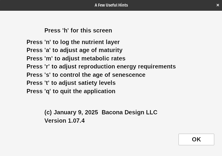
Press 'h' to get this help file
'd' hides/shows the population data shown in the upper right of the display
'l' saves a sample to disk to sample9GM.dat choose 1000 each of P, H, C from the population
'n' logs the nutrient layer to nut.dat save energy level at each 3500x3500 E(i,j)
'a' triggers the adjust age dialog box to modify maturity gene offset levels
'm' triggers the adjust metabolic rate dialog box to manage the offset to the energy gene
'r' triggers the adjust reproduction energy requirement dialog to change the floating point factor
's' calls the senescent age dialog box to modify an offset to the senescence gene
't' to adjust the organisms' satiety levels by an offset to the satiety gene
'q' quit the application
I had forgotten these keys only work while the help list is NOT displayed. Notice also that the word PAUSED is displayed below the population data in the upper right when: a, m, r, s, or t dialog boxes are triggered. You cannot adjust these properties if the simulation is running. If you did the program would crash. Trust me, I know :)
Two-click sample mechanism
Scroll to an 'interesting' population feature; an area with many plants and few herbivores, or an area of many carnivores in a herd of herbivores. Once your feature is centered click once to the upper left and again to the lower right. A dialog box will appear with a number of choices to display histograms of genetics, or population counts, to genetic markers, and energy levels. Follow genetic changes using Compare or Spine War. They both compare genes in the sampled populations. Once you are done with the sample discard it by hitting the 'I Am Done with This Sample' button. Notice the simulation does not stop during this sampling technique. Many more features will be added here.
Gnuplot from dt.dat
Gnuplot is an application which graphs data. Freeware versions are available for the Linux, Macintosh, and Windows operating systems. I use the dt.dat file to store time stamped population data. The following scripts plot three of the columns of dt.dat as lines on a graph. Here are the steps used under Linux, from a terminal window. Type gnuplot to start the application. Then type the following (or just cut and paste it):
plot 'dt.dat' using 1:4 title 'Carnivore' with line, 'dt.dat' using 1:3 title 'Herbivore' with line, 'dt.dat' using 1:2 title 'Plant' with line
or the same script with a different ordering: plot 'dt.dat' using 1:4 title 'Carnivore' with line, 'dt.dat' using 1:2 title 'Plant' with line, 'dt.dat' using 1:3 title 'Herbivore' with line
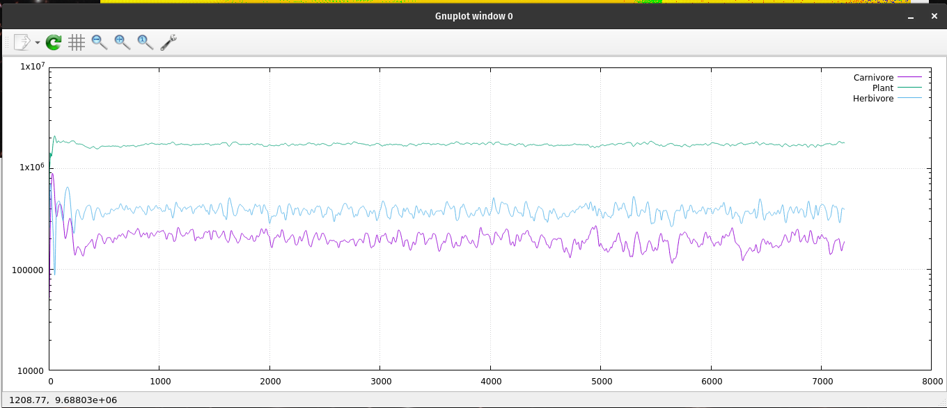
I will parse the last line for you: plot calls the 2D graphing system of Gnuplot. It reads dt.dat as its data source. Using 1:4 tells the 2D system to use column 1 as the X coordinate, and column 4 as the Y coordinate. Title names what you want on the graph's legend; in this case 'Carnivore'. With line draws a line from one data pair to the next. This pattern is repeated for the herbivores and plants. I use the second ordering now because it displays plants as green, herbivores as blue, and carnivores magenta, better fitting their respective natures.
Plot displays a linear graph. If you want log, or log, log scales try these commands:
set logscale y leaves the X coordinate alone while it maps the Y coordinate logarithmically.
Type set logscale for a log, log chart where both X and Y are displayed logarithmically.
Depending on your data set characteristics, each setting can be useful.
To return to a linear plot type unset logscale.
The Chromosome Map
EN::{ senescence, maturity, satiety, absorb, energy }. Senescence limits organisms to a finite life time, maturity allows time to gain energy and it limits the birth rate, satiety prevents an organism from eating more than it needs, absorb is the amount of energy an organism receives from its food source, and energy is the metabolic rate.
PL::{ strength, spine, pollen } Strength determines the amount of poison, spine controls the length of spines, and pollen determines the pollination rate.
HB::{ camo, eat, resist } Camo controls the efficiency of camouflage, eat allows consumption of some level of plant poison, resist limits the length of spines you can eat.
DR::{ speed, SE, S, SW, W, NW, N, NE, E } Speed limits how far an animal can travel in one time cycle, the direction genes determine the direction probabilities.
SN::{ sight, hearing, smell, taste, touch } Six bits each for all five senses. Still a work in progress.
CN::{ attack, range, sleep, camo, pursuit } I have not implemented any of these behaviors yet.
This gene map is subject to change.
Origin stories
Microcosmic God by Theodore Sturgeon
January 28th, 2025
I rewrote ecoDraw.c so it loads 'nut.dat' and 'sample9GM.dat' if they are available. If they are not in the current folder ecoDraw.c generates two random sets of data. Then it creates a population of plants, herbivores, and carnivores using samples from both data sets. Currently it creates one half from one data set and the other half from the second data set. I plan to let the user inject new organisms during the simulation. The genetic marker chromosome GM is on each species. I have one data set marked as 3855 = 0000 1111 0000 1111 and the other set as 61680 = 1111 0000 1111 0000. I chose the numbers to contrast their binary representations. You can mark them however you wish. More tools to write :)
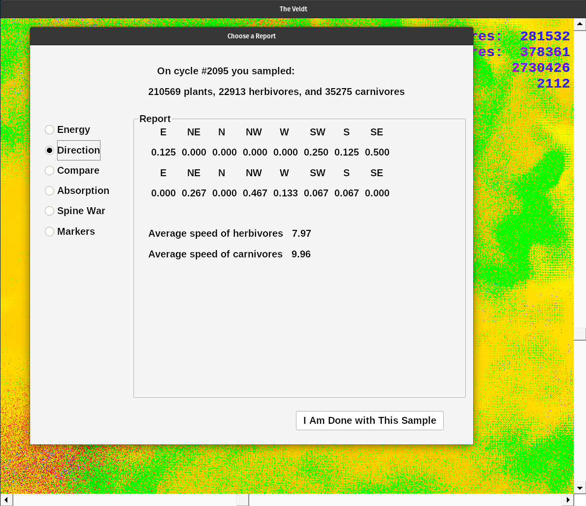
Previously I used readSamples.c to get a report. Now I have implemented that code inside ecoDraw.c. Find an interesting group of herbivores and carnivores on the display. Click above, and to the left of the center of interest. Click again diagonally across the feature. After the second click, a report dialog box appears. Currently there are six report options in a row of radio buttons. The choices include: energy, direction, compare, absorption, spine war, and markers.
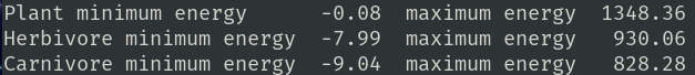
Energy displays the average plant metabolism, average absorption coefficient, average satiety level, average senescent age, and minimum, average, and maximum age of plants.
Direction displays the normalized direction probabilty vectors of herbivores and then carnivores. These are not histograms, but coordinate values of the probability vector. Next their average speeds.
Compare displays the minimum and maximum energy values for plants, herbivores, and carnivores. Then it compares a few competing genes. Poison level versus poison resistance. Then camouflage effectiveness versus visual acuity. Lastly spine probability versus ability to eat spines. I chose these genes to see how they populations changed over time. I found herbivores could gradually eat higher levels of poison. But I also found carnivores with excellent eyesight dominated quickly. I used the spine vs ability to eat spines as a control group. Since I had not implemented the choice in the eating algorithm there should be no tendencies in either gene. This choice is mirrored in spine war. Here you see the percentages change over time. I created histograms in the spine war report.
Absorption introduces histograms. I determine the end points of the values of each trait. Divide the result by ten and use it to create the bins of histogram. I calculated the value of each trait, counting how many fit into each of the bins. Here I have the plant energy absorption coefficient histogram. This shows how much energy each can absorb from the nutrient layer during each cycle. Next, the herbivore energy absorption coeffient histogram. This displays the same trait for herbivores. Lastly the carnivores histogram. Use the reports to track certain traits over time.
Spine war displays the camouflage effectiveness, visual acuity, poison strength, poison resistance, spine probability, and spine eating histograms. Click on Compare to check the similarities.
Markers displays how many plants came from the PS or the PB buffers. Restart ecoDraw.exe with 'sample9GM.dat' in the folder. Make sure it is from a long simulation run so the chromosomes have been highly selected. Then rerun the application. After a few hundred cycles take a spot sample and compare their genetic markers. The 'mature' genetics should far outnumber the new, randomly constructed organisms.
A random selection from the population is stored every 50 cycles. It is called 'sample9GM.dat'. If you press N you save the 'nut.dat' file, a copy of the nutrient layer. Start ecoDraw.exe with one or both of these files present. Random populations on a mature nutrient layer is a good choice. Or use the sample file for mature genetics on a uniform nutrient layer. Or, if you have both 'nut.dat' and 'sample9GM.dat', you are using a mature nutrient layer with a highly selected genetic population of organisms. It is up to you, and how you wish to experiment. When you are done reading reports click the dialog's only button, or hit the enter key to exit. Notice this dialog does not block the execution of the simulation. You can read each report as they ecosystem continues without pause. Keep track of the gene competition by taking spot samples and reading the reports. Have fun!
January 9th, 2025
I have expanded readSamples.c to create longer reports. Instead of reading the data randomly sampled every 100 cycles, I wrote a new routine. Click on a point bounding an interesting growth feature. Then click diagonally opposite from the first point. That creates a spot sample file of all the plants, herbivores, and carnivores inside the rectangle you chose. Now that you have 'spot.dat' you can analyze it by typing ./rs (if you have compiled readSamples.c < g++ -o rs readSamples.c > ).
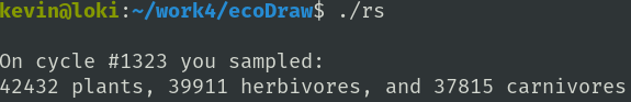
The report begins with the present cycle count. Each cycle is not really a time unit. It is not a generation and it is not a day. It is one cycle through the ecosystem loop: move, metabolize, eat, reproduce, die. One organism can live as little as one cycle, or as long as ninety cycles. The former organism was probably eaten while the latter is close to senescent. It is good to choose a large number of all organisms. This gives a better spot sample. I wanted to track the traits of 'herds' of herbivores or carnivores. Or track the ages of a meadow of plants. Or compare the energy levels of the organisms to the energy level of the nutrient layer.
Plants, herbivores, and carnivores have traits which compete with one another. For instance: plants have a poison strength gene, while herbivores have a gene which allows them to eat some level of poison without harm. Herbivores also have a camouflage effectiveness gene which competes with the carnivores' eyesight gene.
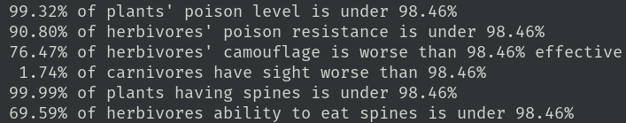
The next two genes are chosen as a null test. Plants have a gene for spine presence and herbivores have a gene which allows them to eat some level of spines. I did not express this limit in the code, so they are not in competition. However, while the carnivores select for the very best eyesight, and herbivore's resistance to poison grows better, plants don't select for more poison at the same rate. Neither do herbivore select for only the best camouflage. These two genes improve around the same rate as do the un-competitive genes. Hmmm...
I wondered if there was any bias in direction choice so I created a tool to test this. The tool is now incorporated into readSamples.c. It produces this report:
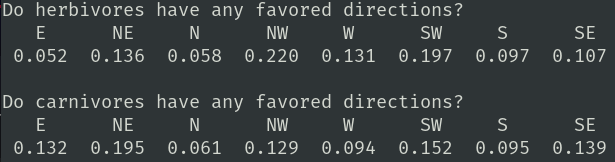
Each herbivore and carnivore has a DR chromosome. Each chromosome has nine genes mapped onto it. Eight genes, of 3 bits each, represent eight points of the compass from E to NE to N to ... to SE. I sum the value of each gene then go back and divide each raw value by the total. This gives me a normalized direction probability vector. A perfectly balanced animal would have 0.125 in each bin. It is interesting to see how separate 'herds' have different direction biases.
Lastly there are lists of average values from plants, herbivores, and carnivores in your sample.
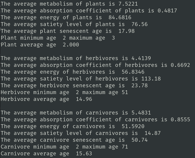
I am using this report to modify the gene expression coefficients. Presently I have no idea why plants have an average senescent age of 17.98 but rarely get more than five cycles old. I also don't understand why the metabolism of plants is higher than either herbivores or carnivores. I need someone more familiar with the energy flows than me. Spot sampling has been instructive. I have removed, and then reinstated senescence for all organisms. Without it the population levels grew too fast and too large. There are over forty parameters which can be changed to modify the system's health. Hopefully someone will find this interesting enough to continue my quest.
I created a better help window. Press the 'h' key to get:
The dialog lists some of the parameters which can be changed during a simulation. You can only modify the population levels at the start. Otherwise all other parameters can be modified. Press the correct key to pause the simulation while you make changes to a parameter or two. Once you hit OK or Cancel the simulation resumes where it left off. The help dialog box does not pause the application. If you press 'n' you log the current nutrient layer to nut.dat. This file is useful to start the ecosystem with a varied nutrient layer. When you place new organisms on top of this some do very well, while others perish from lack of nutrients. A uniform layer of nutrients shows another growth pattern which favors different genetics. The spot sample reports are quite useful to adjust the framework.
December 18th, 2024
I created S4L5_Ecology using C++. S4L5 was useful for learning how to use C++. It showed me the good parts and those which are less useful. C++ worked OK but it did not scale well. I could not get to 1000 x 1000 cells.
How it began: Ecology.pdf
S4L5 Lesson: S4L5_ecology.pdf
S4L5 executable: eecology.exe
Then I wrote ecoNode.c using C. I recreated my simulation using a few techniques I have developed. Buffering helps organize and accelerate the app. Simplifying indexing made writing the code much easier. I can work with a 2D E(i,j) ecology cell or a 1D PL(i) plant node. Once I got the addressing framework developed and debugged I was able to increase my problem space first to 3000 x 3000 and then to 5000 x 5000 where it is set now. The new tools let me breed many more organisms. 2 million plants is not uncommon, nor are 500 thousand herbivores, or 200 thousand carnivores. I have had stable ecosystems working beyond 250 thousand cycles.
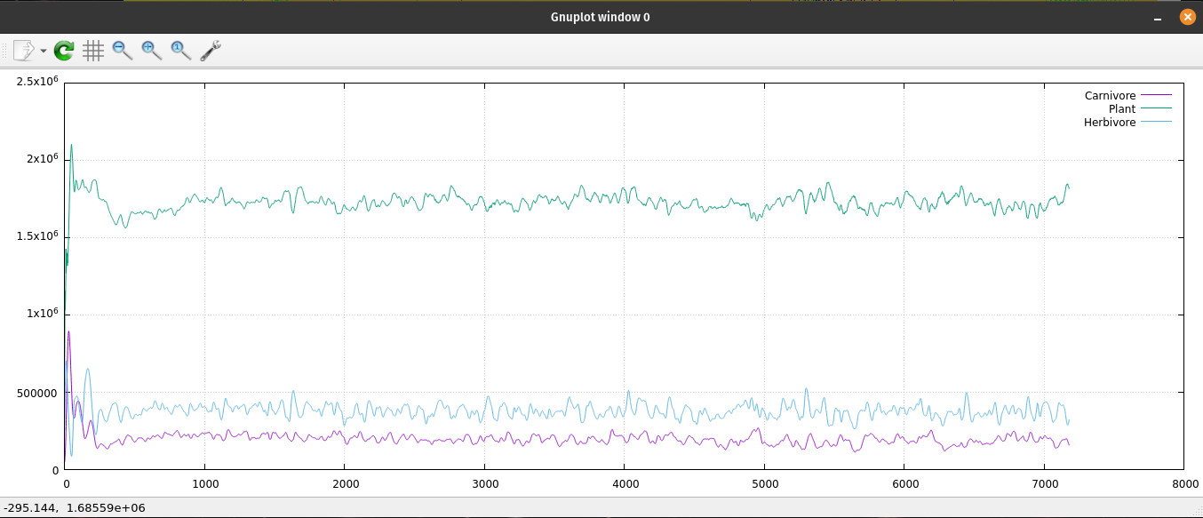
Since ecoNode is a command line application, I needed a way to monitor the population levels of the ecosystem. I have been using gnuplot for many years; I enjoy its simplicity and ease of use. I generate many data files to monitor my code. I use gnuplot to read those files and create 2D graphs. It naturally plots with linear x, y coordinates. If I type "set logscale" I get a log-log chart of my data. Or type "set logscale y" to get a semi-log chart. Each chart has its uses by showing some characteristics better than others. I tried 'set logscale x' and found another way to look at changes over time. gnuplot is very useful to have on your computer. My normal procedure is to open two terminal windows pointed at the same file location. One of them is running my application generating a data file. The other terminal window is running gnuplot which reads that data file and generates a 2D chart.
Find gnuplot here: gnuplot
A plot of the ecosystem's population data.
A log log plot of the ecosystem's population data.
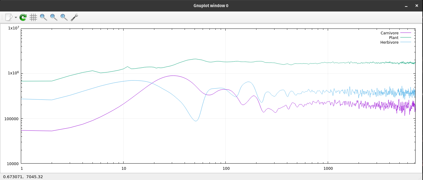
A semi-log plot of the ecosystem's population data.
I implemented many values as floating point where they had been integers in S4L5. Tracking the energy flow through the environment is easier. That allowed me to determine how much energy was being lost to metabolism, or through senescent organisms. Once I knew those values I could replenish exactly that much back to the nutrient layer.
ecoNode: Ecosystem_simulation.pdf
ecoNode source code: ecoNode.c
ecoNode Linux executable: en
ecoNode Windows executable: en.exe
I reused code from a graphics template I've built. I modified the main loop of ecoNode.c so it would run as a thread in a Windows application. I wanted to retain the speed of the ecological engine, so I created another thread to display the ecosystem. I did not want to slow down either one by synchronizing them. So there are glitches. However, they are few at first, then almost non-existent once the simulation has matured. Since they work in a producer consumer symbiosis they can get out of sync. Especially when population counts drop during the first two hundred cycles. Once, and if, the ecosystem recovers equilibrium, cycles require over a second to complete. Modifying the bitmap takes about one second. When the producer creates frames faster than the consumer can display them you will see the cycle count jump erratically.
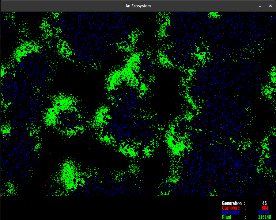
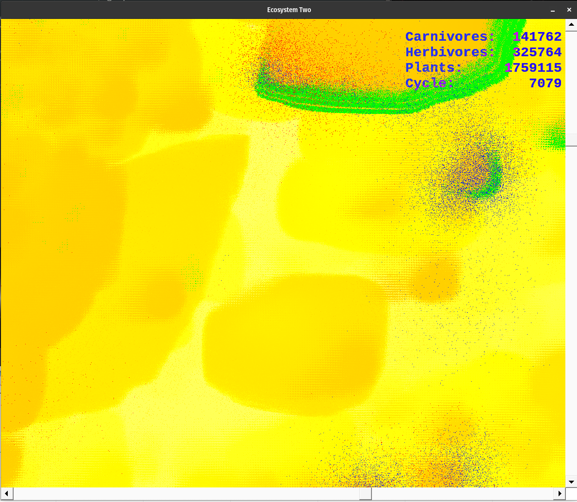
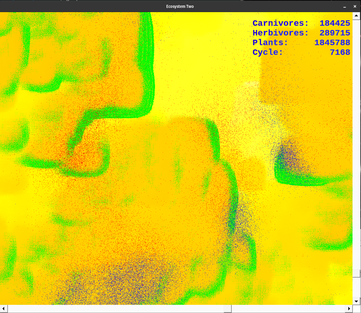
The background bitmap is 5000 x 5000 pixels square. 25,000,000 pixels take a while to change. My foreground display is a window onto that background bitmap. You can move the display around by scrolling the mouse, using the scrollbars, or by using the arrow keys on the keyboard. The display does not scroll smoothly; there are blanks. This is also due to the size of the background bitmap. I need to work on this; but it recovers quickly. The data display is a small, separate window which is blitted on top of the ecosystem window. I fill that window with black and draw the text on top of it. Then I blit it using the SRCINVERT raster operation. Notice how the color of the letters change as the underlying image changes. This is especially noticeable when a herd of herbivores pass underneath the numbers. It appears they are eating the legend :)
The colors designate various things. The gradient from dusky orange to white is the amount of energy in the nutrient layer. Brighter points have more energy than the dusky orange ones. Notice what happens when plants pass through an area as they go through their life cycle. Energy is lost via metabolism and through the death of senescent organisms. This amount of energy is evenly spread back to the nutrient layer. Over the cycles, some areas get so energetic they pass beyond my color palette. They indicate as black dots. When plants grow over them they breed rapidly. However, the herbivores always seem to find them before they're done feeding on the available nutrient energy.
Plants are green, herbivores are blue, and carnivores are red. When they overlap they produce shades of violet. The color palette for the nutrient layer starts at blue, goes to red, then yellow, and finally white. I chose the lowest color I could and still have enough contrast to see the carnivores. The topmost color is white, which is set at 6000.0 energy units at present. When the energy level exceeds 6000.0, the pixel turns black. However, this does not happen too often. If it does change the upper range of the color palette in colorTransform().
I am going to continue work on the user interface, and work on sampling and marking tools. I will probably add a tool to create 'synthetically' created sample files. That will let the user modify the individual genes of each chromosome of an organism. Then clone one thousand of them and add them to a stable ecosystem. Use the GM chromosome to follow your new organisms as they live and breed. Lots of other fun things to do. Like expressing more genes to give the herbivores and carnivores more behavior. I have a sensor net idea which would help the carnivores find herbivores more easily. Either by scent or hearing or sight. I'm not sure which; the ideas are working themselves out.
Plants, herbivores, and carnivores have many traits which are genetically determined. Some of the 36 tweakable parameters are an offset to a gene value. Instead of looking at genes solely as integers, I implement them as floating point values, or as factors between 0.0 and 1.0. For instance: if my gene is four bits long, its raw value can range from { 0 .. 15 }. Using zero is not good, it can lead to problems. So I add one to get the range { 1 .. 16 }. If I divide the raw value plus one, by 16, I get a range of { 1/16 .. 16/16 } or { 0.0625 .. 1.0 }. That is good for something like the absorption rate. For instance, a plant can gain 5/16 of the nutrients available in the cell. If I use a factor here, instead of a set amount, I avoid negative numbers. 5/16 of very little is still very little, but not below zero. When I saw the first images from ecoDraw I was reminded of paintings by Joan Miro. The palette was not chosen to that end, I think :)
Some of the user tweakable parameters are offsets from the gene value. Say your gene is 3 bits long, which ranges from { 0 ... 7 }, instead of using an offset of 1, use 3 to get a range of { 3 ... 10 }. Use casting to make these values floats instead of ints. Remember: 10 bits gives you 1024 steps, 8 bits gives you 256, and 3 bits gives you 8 steps. Build your genes to fit your problem settings.
A rudimentary gene map: geneCruft.c
ecoDraw.exe was compiled under a Windows 7 environment. It will run fine on any Windows machine of that era or newer. The application requires 1.3 GBytes of memory. It also employs three threads of execution. Two threads run at ~100% duty cycle, the third thread is for the UI and requires little processing time. Fast, multi-core machines work best. One of mine is creating one frame every two to three seconds. Your mileage will vary. One thousand cycles an hour is good.
ecoDraw: ecoDraw.pdf
ecoDraw source code: ecoDraw.c
ecoDraw executable: ecoDraw.exe
I rewrote ecoDraw.exe so it can start without any other files. It is more boring, and the ecosystem thus created will likely crash. If you have sample9GM.dat you are using organisms bred over many cycles. If you have the nut.dat file you are using a mature nutrient layer which displays a wide variation of energy levels. This creates an ecosystem from data sampled during long simulation runs. Without it the system is populated by organisms with random sets of chromosomes. A few boom, bust cycles follow. If you are lucky, the carnivores will not die out and your simulation will stabilize.
I normally work from a command line in a terminal window under a Linux OS. Any debugging or logging operations go directly to this terminal window. In Windows parlance this is a command window. If you launch the application from the Windows file system it will create a display window then open a terminal window. I use the data flashing by to monitor the energy condition of the ecosystem. If it is too annoying I can change the compiler flags to turn it off. I just want you to know a command window will appear.
If you are running a Macintosh, or Linux, operating system the Wine translator works fine with my code. I use Virtualbox to compile in a Windows 7 environment. Then I run the executable under Wine so each operation has been tested many times. I have not tried running my code on a Mac. I would like to hear how it works for you.
Find wine here: wine
When you start the application you are presented with a series of six dialog boxes, with three choices each. I recommend you hit ENTER for each of them, to use the default settings, until you get a feel for the program. During any run you can hit the 'h' key for a help list of your options. I implemented a keyboard UI instead of using menus. They are simpler and take less screen space. While the simulation is running you can change a few settings. Call up your chosen dialog box and the simulation will pause. Modify a setting and hit OK, or CANCEL. The simulation will resume running with your change(s) intact controlling the ecosystem's destiny.
There are a number of non-linear relationships, so the parameters may be finicky. Often the effects of a change will not be visible for many cycles. Monitor the system health by using gnuplot on 'dat.dt'. Chart both the population levels and maximum energy levels for a good idea of what's going on. If you see a steady decline in population over a few thousand cycles there may not be enough energy in the system. But, too much energy is also a problem. Change the parameters carefully, and with forethought to achieve good results. Sometimes the settings are counterintuitive :)
Incrementing settings one click at a time is tedious. Use the tab key to choose the up, or down, arrow you want. Then if you hold down the ENTER key you can change the value much more rapidly. Tab to the next arrow key and repeat. Laziness, Impatience, and Hubris are three great virtues :)
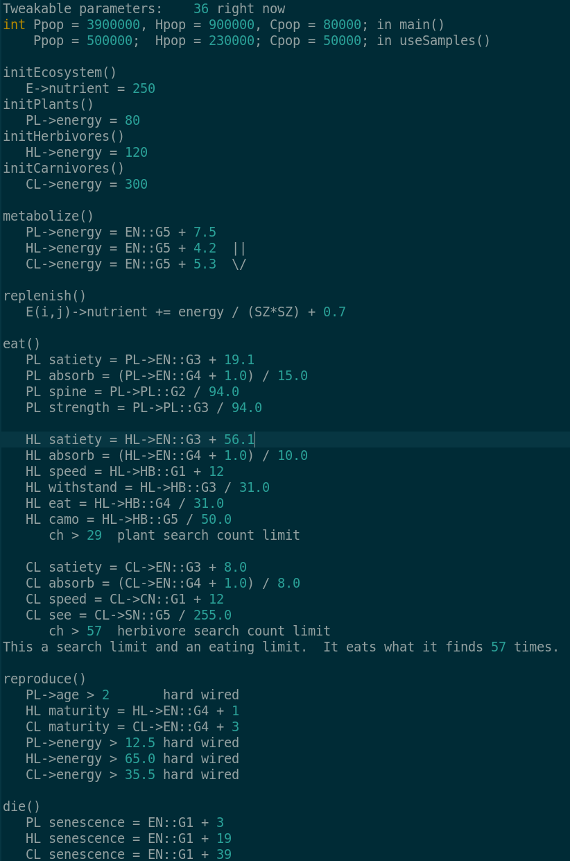
Currently Tweakable parameters:
int Ppop = 500000, Hpop = 230000, Cpop = 50000;
float PRenergy = 12.5, HRenergy = 65.0, CRenergy = 35.5; // Reproduction energy level hard wire
int PNoffset = 3, HNoffset = 19, CNoffset = 39; // Senescence - EN::G1 + offset
float PSoffset = 19.1, HSoffset = 56.1, CSoffset = 8.0; // Satiety - EN::G3 + offset
float PMoffset = 7.5, HMoffset = 4.2, CMoffset = 5.3; // Metabolism - EN::G5 + offset
I added the GM chromosome to each organism. Previously, only plants had it. GM contains 31 bits of information. I use it as a marker to trace inheritance. The GM chromosome is passed directly by the mother organism without any crossover. I have been using it to see which genes compete better than others. Or a random population compared to a mature population.
When I had the genetic marker chromosome in place, I needed tools to analyze my sample files. The first thing I did was count how many plants had a genetic marker as a percentage of the whole population. Then I generalized extracting genes from chromosomes. I created a data structure, gmap, which holds the mask and the shift amount, for each gene in a given chromosome. This has to be mapped by chromosome by organism since they are not all the same.
I wrote readSamples.c to display chromosomes and extract genes. Once you extract the raw data you need to transform it into integers or floating point numbers. Each type can have offsets and divisors. I wrote the function compareGenes() to examine the competition between a plant's poison level and the ability of a herbivore to resist poison. Or the ability of a herbivore to hide from a keen sighted carnivore.
Every 50 cycles I randomly sample the ecosystem for 1000 plants, 1000 herbivores, and 1000 carnivores. I store their genes, energy levels, and ages for analysis. I use readSamples() to read the organism data in sample9GM.dat. I want to automate this because I am seeing some interesting changes. For instance, the simulation selects only carnivores with excellent sight. It also breeds for herbivores which the ability to resist poison at the highest levels. Conversely, the plants breed higher poison levels, but they do so very slowly. Similarly, the herbivores breed for better camouflage rather slowly.
A random sample of plants, herbivores, and carnivores is collected and stored every 50 cycles. I wanted to sample interesting groupings from the simulation while it was running. So I created a spot sampling method. Display buffering prevents me from drawing the characteristic rubber band selection scheme. But I can capture two clicks in order. If the user did not sweep from upper left to lower right I flip the coordinates in the code. The two click points select a rectangle from the E(i,j) ecosystem. The function scans the rectangular area counting, and logging organisms. I have not written the tools to read and analyze the data collected. I am using it for spot population counts. You can open spot.dat in an editor and update it each time you pick a new rectangle. I need to expand readSamples.c with its own user interface. Then it can compare genes more easily.
You can store the nutrient layer at any time by hitting the N key. This stores nut.dat which is a map of the current nutrient layer. I let one of my laptops run ecoDraw.exe for long periods of time. They can go to sleep so I have runs over a week long. I have been saving nut.dat from them. However, I rewrote ecoDraw today so you don't need nut.dat, or sample9GM.dat, to get started. If the application doesn't find either, or both of them, it places random organisms on a uniform nutrient layer. If you can get the system to run until it becomes stable save the nutrient layer and a sample9GM.dat file for the future.